Quick Start Guide

Introduction

This guide provides step-by-step instructions for depositing a simple thin-film morphology and performing electronic structure analysis on it using Nanoscope. It is designed to help you quickly get started with the basic functionalities of Nanoscope. For more complex use cases, please refer to the User Guide section.

Prerequesits

• Nanoscope Installation: Ensure that Nanoscope is installed on your system. If not, follow the Installation to set it up.

Production Run vs. Test Run

Below, we provide settings for each module in the Nanoscope workflow. Each module includes configurations for two types of runs: Production Runs for meaningful and accurate results, and Test Runs for quick checks of workflow functionality and output.

Production Runs	Test Runs
Settings for production runs, resulting in meaningful, accurate results.	Settings suitable for quick technical tests that deliver quick (but meaningless) results also on small computational resources.

Refer to the installation guide for recommendations for hardware and software setup for production runs and quick technical tests.

Simulation Setup

a. Design and Download the Molecule.

1. Open MolView in your web browser.

2. Design a molecule of your choice, e.g. a biphenyl molecule.

3. Use the clean and the 2D to 3D buttons to generate a 3D structure of the molecule.

4. Download the 3D molecule file with Tools -> MOL file.

   

   Design a molecule with MolView

Note

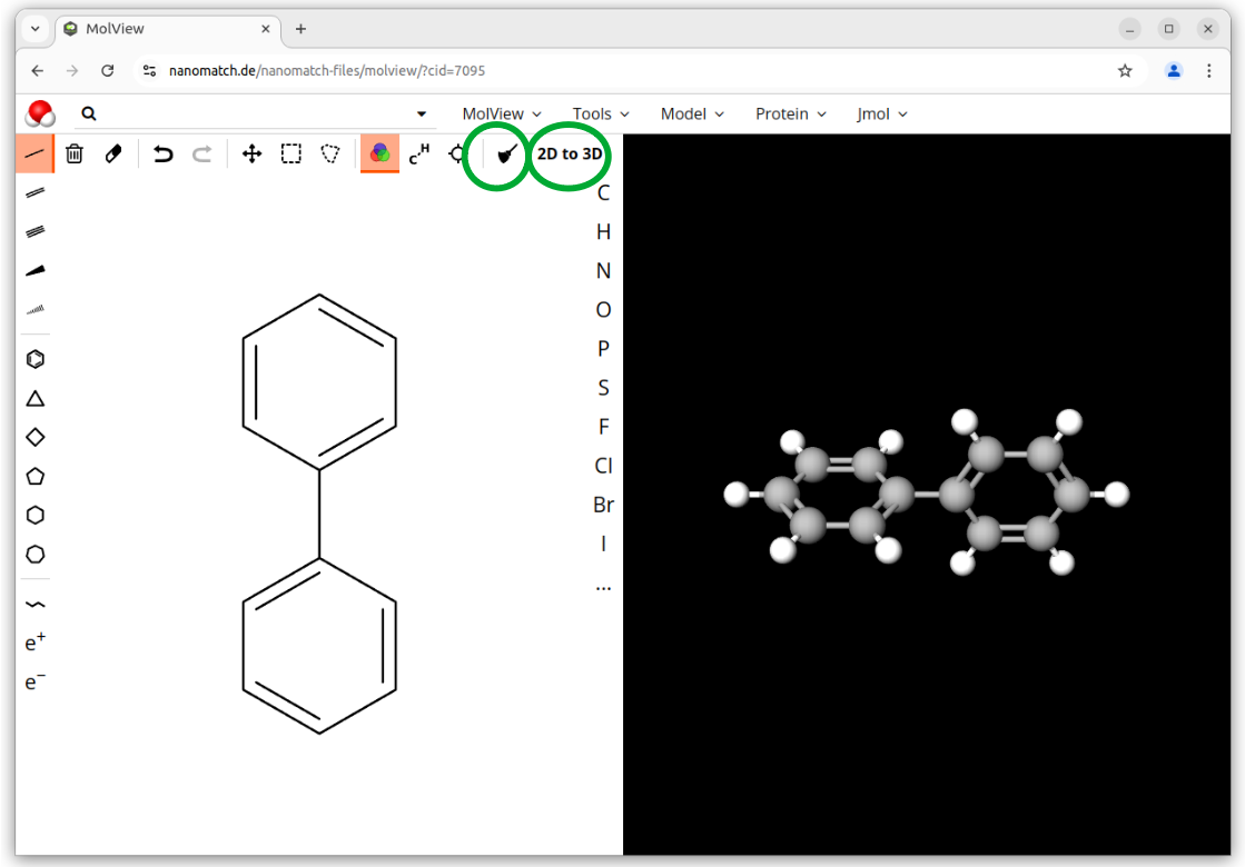
We use biphenyl as a simple example as it allows for quick computation. It is not meant as a physical case study. Feel free to try a different molecule. Keep in mind that the basic usage of Nanoscope covers molecules with up to 40 atoms.

b. Launch SimStack.

On your local PC do the following:

micromamba activate simstack
simstack

This will activate SimStack environment and launch SimStack.

c. Set Up the Basic Nanoscope Workflow.

Drag&Drop the modules MolPrep, Deposit and ESAnalysis from the top left panel into the middle workflow panel into a linear workflow and arrange as depicted below. Double click on each module to adapt settings and allocate resources for each simulation step.

d. Set Up Individual Modules

In the central panel, double-click on the module to set it up.

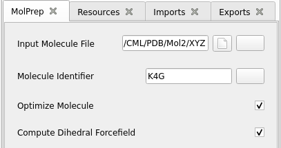
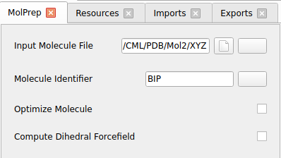
1. MolPrep.

   • Set the Input Molecule File: select the molecule you created above.

   • Only for test runs:

     • Disable Optimize Molecule

     • Disable Compute Dihedral Forcefield

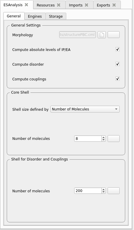
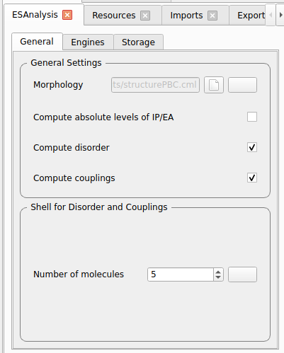
   Production runs	Test runs

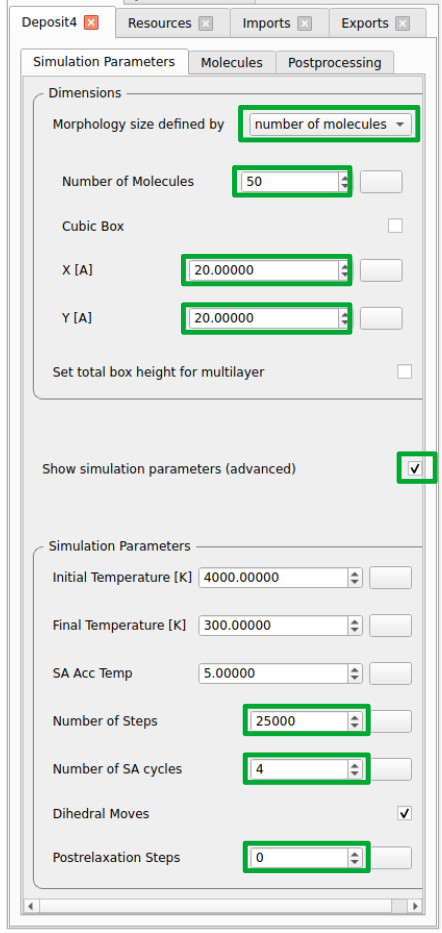
2. Deposit

   • Adjust the Simulation Parameters tab as indicated in the screenshots below. Note that for a standard production run, the preset simulation parameters can be used without adjustment.

   Production runs	Test runs

   • In the Molecules tab:

     Click on the rightmost buttons next to the input fields to load molecule and forcefield file from MolPrep:

     • Molecule input: MolPPrep/outputs/molecule.pdb

     • Forcefield input: MolPPrep/outputs/molecule_forcefield.spf

     Note

     The *.pdb/*.spf files above do not yet exist; you specify the file paths where MolProp module will generate them.

     The video below shows how to load the molecule and force-field files:

   Click to animate

3. ESAnalysis

   • In the General tab of the ESAnalysis module, adapt the following:

     • Morphology: Deposit3/outputs/structurePBC.cml (again using the rightmost button)

     • For Test Runs only or if the absolute energy levels is not important:

       • Disable computation of absolute values and compute disorder and couplings only for a small shell

   Production runs	Test runs

   • In the Engines tab, set Memory per CPU to the total memory of your compute node divided by the number of processors.

   Production runs	Test runs

e. Set Up Resources for Every Module

For each module, go to the Resources tab and set the computational resources:

• For test runs using test-settings as indicated above: Use whatever you have available

• For production runs, the following is recommended:

  Module	CPUs	Memory (MB)	Walltime
  MolPrep	≥32	≥64000	A few hours
  Deposit	32	≥64000	A few hours
  ESAnalysis	≥64	≥128000	Several hours

Please do not forget to set up resources for each and every module in your workflow as animated below.

Click to animate

Note

• You can run the workflow with fewer cores, if the above resources are not available. This increases runtime respectively.

• Memory is provided in MB in the Resources tab. Running Nanoscope with less memory than indicated in the table above is possible, but you may run into out-of-memory issues especially for larger molecules.

• Walltime is provided in seconds in the Resources tab.

f. Save and Submit the Workflow

1. Save the workflow with Ctrl+S or by clicking File -> Save or File -> Save As...

2. Connect to your resource using the Connect button in the top right of SimStack. Wait for the button to become green.

3. Submit the workflow wiht Ctrl+R or by clicking Run -> Run.

g. Monitor Progress

You can monitor the progress of your workflow with the Jobs & Workflows tab in the right panel of SimStack:

1. Navigate to the Jobs & Workflows tab on the right panel.

2. Expand Workflows (double click) and locate your submitted workflow (identified by timestamp if necessary).

3. Monitor the status of the workflow and the contained modules:

   • Green: Completed successfully

   • Yellow: Currently running

   • Red: Encountered an error

4. Double-click on a module to view logs, output files, and detailed status.

Note

Modules are only listed in this view once they have been started, i.e. when the predecessing module was finished successfully.

5. Analyze output with one of the two options:

   • Right-click on a workflow or a module and click Browse workflow or Browse directory to browse output files in a web browser.

   • Download individual files to your hard drive by double-clicking on the respective file in the panel depicted above.

Output

Here we present a few examples of outputs of the standard Nanoscope workflow. For a detailed description, refer to Computed Properties or Examples.

MolPrep Output

File	Content
output_molecule.mol2	coordinates of the optimized vaccum conformation
molecule.pdb	optimized molecular vacuum conformation, formatted for Deposit
molecule_forcefield.spf	forcefield file for Deposit
mol_data.yml	HOMO, LUMO and static dipole

Deposit Output

File	Content
structure.cml	3D coordinates of the atoms in the thin film morphology. This file can be visualized with jmol
structure.mol2	Atom coordinates in mol2 format
structurePBC.cml	Morphology extended periodically in x- and y-direction, lateral to the deposition axis
summary_RDF.png	Plot of radial distribution functions of molecular center-of-geometry (COG) positions
visualization_2D_and_3D.png	Visualization of molecular COG positions
output_dict.yml	Raw data of radial distribution functions, density (in g/cm3) and simulation settings

ESAnalysis Output

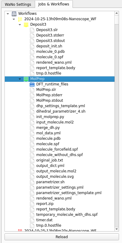
The primary outputs of the ESAnalysis module are located in the Analysis/DOS directory within the module’s runtime folder.

HOMO and LUMO distribution in a pristine morphology. The values in the figure are onsets of the distributions that compare to experimental values.

Further outputs are:

File	Content
DOS_Gaussian.png	Plot visualizing the Gaussian-broadened density of HOMO and LUMO levels without vibrational effects.
Vibrational_Gaussian_DOS_plot.png	Plot showing the Gaussian-broadened HOMO/LUMO distribution including vibrational broadening.
all_DOS_plot.png	Combined plot overlaying DOS distributions with and without vibrational broadening (both are Gaussian-broadened).
raw_data_homo_lumo.yaml	Exact HOMO and LUMO energies (in mixed morphologies for each molecule type). Includes mean, std, and all individual energy levels.
homo_lumo_onsets.yaml	Calculated onset energies for HOMO and LUMO levels distribution for each molecule type, can be compared with experimental onsets.
homo_lumo_centers.yaml	Mean and standard deviation of the distribution of HOMO and LUMO levels for each molecule type. Can be used as an ab-initio input for multi-scale simulation workflows.