Computed Properties

Overview of Property Groups
MORPHOLOGY Morphological Structure Density Radial Distribution Function (RDF) Molecular Arrangement	POLARIZATION RESPONSE Dielectric Permittivity Polarization Energies
EMBEDDED MOLECULES Ionization Potential (IP) Electron Affinity (EA)	CHARGE TRANSPORT Charge Carrier Mobility Overlap Integrals Energy Disorder

Note

Click on a property or a property group to navigate to its detailed section.

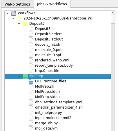
Where are computed properties

In the right panel of SimStack, go to Jobs & Workflows. Completed jobs (shown in green) appear here, organized by the module that generated them, as illustrated below:

Output Structure

Example

Workflows
└─── <TimeStamp><WorkflowName>
     ├── MolPrep
     │    └── ... (files and folders)
     ├── Deposit3
     │    └── ... (files and folders)
     └── ESAnalysis
          └── ... (files and folders)

Morphology

Morphological Structure

Density

Radial Distribution Function (RDF)

Molecular Arrangement

Morphological Structure

Property description

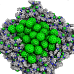
A major output of Deposit are morphologies, i.e. 3D representations of molecular arrangement in thin films with atomistic resolution. These morphologies are the starting point for many types of analysis, ranging from the investigation of molecular arrangement and orientation to the analysis of the electronic structure of molecules embedded in the thin films.

Output files

File	Description
structure.cml	Atom coordinates sorted by molecule in cml format.
structure.mol2	Atom coordinates sorted by molecule in mol2 format.
structurePBC.cml	Atom coordinates sorted by molecule, periodically expanded in x- and y- direction.

Example of `structure.cml` and `structure.mol2` files (visualization)

You can visualize the content of cml and mol2 files using common molecule visualization tools such as jmol or pymol.

Visualisation of structure.cml with jmol:

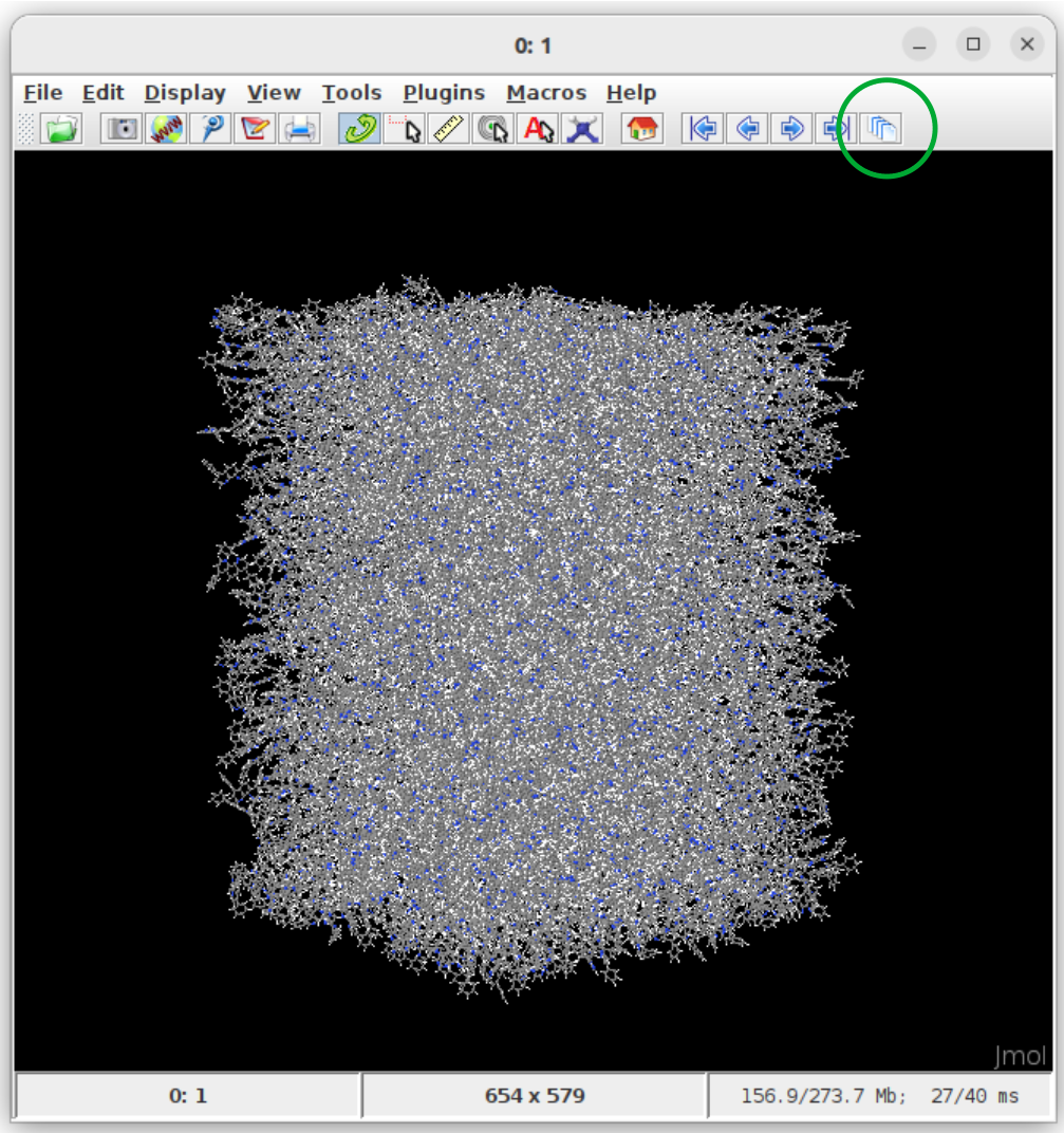
Instructions:

Get jmol from the official jmol page.

In the terminal, move to the runtime directory of Deposit
Open the structure using
jmol structure.cml
Click on the show all frames button (green circle in the figure above).

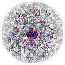
Visualisation of structure.mol2 with pymol:

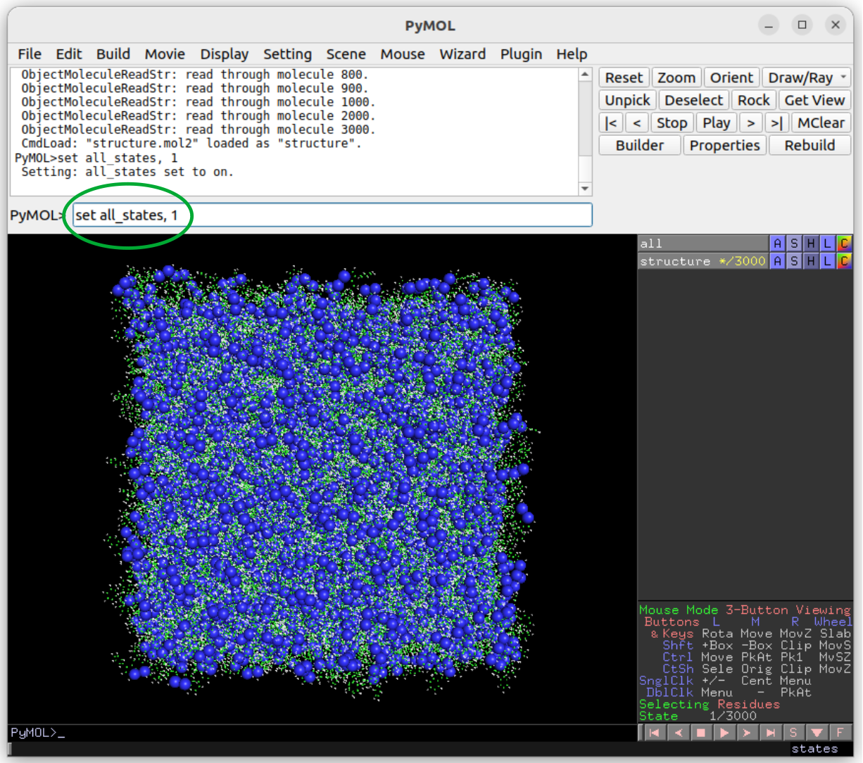
Instructions:

Get pymol from the official pymol page.

In the terminal, move to the runtime directory of Deposit
Open the structure using
pymol structure.mol2
In pymol, type set all_states, 1 to show all molecules (green circle in the figure above).

Density

Property description

Density of thin film morphologies generated by Deposit are computed automatically after deposition. Both mass density (g/cm3) and molecular particle density (1/cm3) as well as average molecular volume (nm3) are computed. To avoid edge effects, both properties are computed and averaged over 20 random boxes in the morphology. Standard deviations are provided along with the values.

Output files

File	Description
output_dict.yml	Mass density and corresponding standard deviation are available at keys averaged_box_density and std_box_dens, provided in g/cm3.
Deposit3.stdout	Standard output of the Deposit run lists the density analysis near the end of the file, lines starting with box density avg over 20 samples. First line is mass density, second line is molecular particle density. Molecular volume is listed below.

Radial Distribution Function (RDF)

Property description

In amorphous solids, the radial distribution function (RDF) describes the probability of finding other molecules at a certain distance from a reference molecule, averaged over all molecules in the material. Molecular positions are specified by their center of geometry (COG). The first peak in the radial distribution function corresponds to the most probable distance between a reference molecule and its nearest neighbors, and represents the average nearest-neighbor distance in the material. In mixed films, RDFs are computed resolved by species.

Output files

File	Description
summary_RDF.png	Plot of radial distribution functions of molecular center-of-geometry (COG) positions. For mixtures, this figure contains plots of RDF between all molecular species.
rdf_{uuid1}_{uuid2}.png	Plots of individual rdfs between types. Exists only for mixed morphology.

Molecular arrangement in thin films: GSP/SOP

Property description

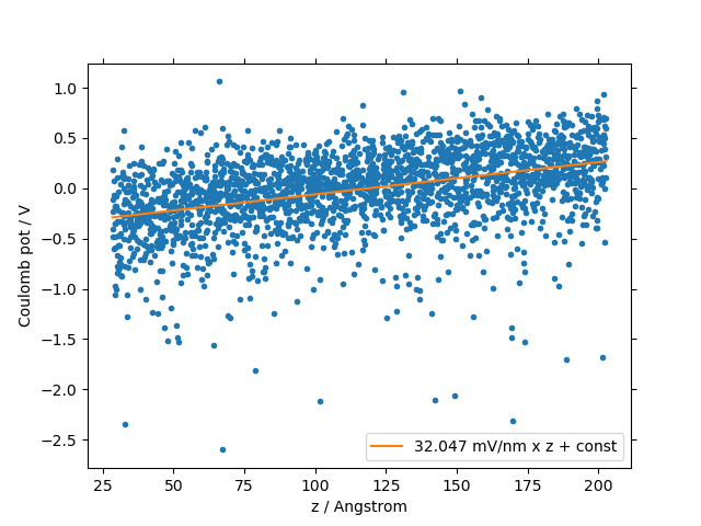
In amorphous solids, spontaneous orientation of polar molecules due to van-der-Waals interaction with the substrate may induce a potential drop across the thin film along the deposition axis. This effect is called spontaneous orientation polarization (SOP), giant surface potential (GSP) or built-in potential. We compute the slope of the potential across (in x- and y-direction infinitly extended) thin films using the orientation of molecular dipoles in deposited thin film morphologies using the GSPAnalysis module. Further details are available in the publications section: Built-In Potentials Induced by Molecular Order in Amorphous Organic Thin Films.

Output files

The GSPAnalysis module prints the value of the potential slope into the standard output, typically named GSPAnalysis.stdout. Further, the figure GSP_analysis_system_scatter_fit.png shows the potential on all molecular sites induced by the spontaneous orientation of all dipoles in the thin film over the z-position, i.e. along the deposition axis, and the fit applied to compute the potential slope. The resulting slope is provided in the legend:

In addition, this module provides the following output files:

File	Description
output_dict.yml	Computed GSP value in mV/nm.
GSP_analysis_system_potential_data.dat	Potential computed at molecule center of geometries.

Polarization Response

Dielectric Permittivity

Property description

Dielectric permittivity is a short terms used for Relative Dielectric Permittivity, and contains only electronic component of the response of the medium.

Modeling Method

Nanoscope calculates the dielectric permittivity using the polarization energy as a function of the polarization shell radius. For details, refer to the paper:

Computing Charging and Polarization Energies of Small Organic Molecules Embedded into Amorphous Materials with Quantum Accuracy,

Output Files

The computed dielectric permittivity results are saved as a YAML file:

ESAnalysis
   └─── Analysis
          └─── DOS
                └─── data
                       └─── dielectric_permittivity.yaml

This file contains the dielectric constant per molecule type and standard deviation of its values for various molecule types.

Example of `dielectric_permittivity.yaml`

dielectric_permittivity:
  value: 3.6  # Dielectric constant
  std: 0.2  # Standard deviation (for multicomponent systems)

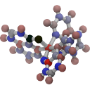
Embedded Molecules

Ionization Potential (IP)

Electron Affinity (EA)

Ionization Potential and Electron Affinity Distributions in Organic Thin Films

Property description

Ionization potential (IP) and electron affinity (EA), commonly referred to as HOMO and LUMO, are computed by the ESAnalysis module on molecules embedded in thin-film morphologies provided by Deposit. The impact of the unique electrostatic environment of each individual molecule is explicitly taken into account. This approach provides:

Distributions of IP and EA (density of states, DOS) in organic semiconductor materials
Shift of IP and EA in guest-host systems compared to pristine films
Band bending at interfaces

… i.e. the investigation of IP and EA on molecules in any given setup.

Note

We will use HOMO/LUMO interchangeably as the negative of IP/EA throughout the documentation where appropriate or commonly accepted by the community.

\[ \begin{align}\begin{aligned}\text{HOMO} = -\text{IP}\\\text{LUMO} = -\text{EA}\end{aligned}\end{align} \]

It is important to note, however, that in some contexts, HOMO/LUMO and -IP/-EA may not be strictly equivalent due to differences in experimental conditions or computational approximations.

Output files

Output structure of the ES Analysis module

Analysis
    └───DOS
          ├───data/   # Directory containing all images.
          └───plots/  # Directory containing all data files

Images in Analysis/DOS/plots

1. all_DOS_asis_plot.png

This is the most comprehensive visualization. The image below is an example for the two-component system CBP:CN6-CP(20 mol%):

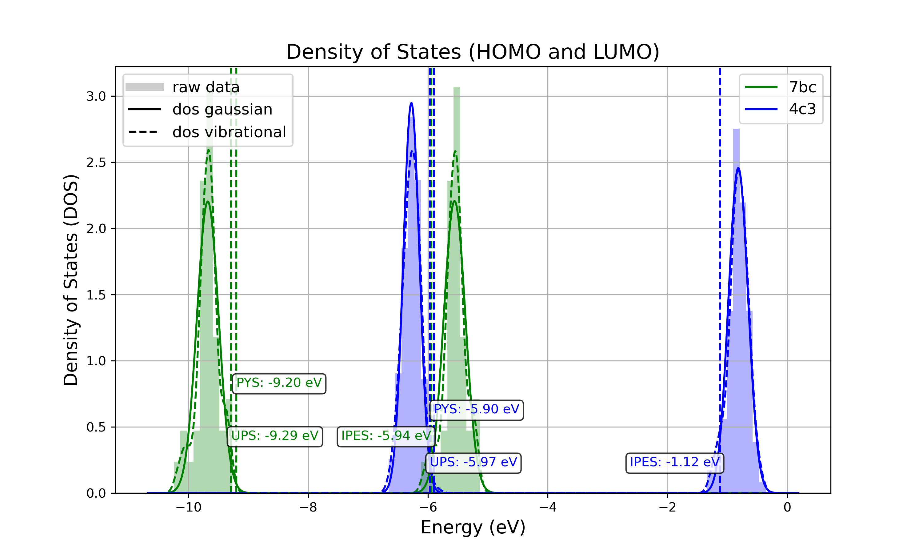
Figure: all_DOS_asis_plot.png - Combined plot showing raw distributions of individual HOMO and LUMO levels, their Gaussian approximations, and DOS distributions with vibrational broadening effects. These are computed from individual energy levels and include onset energies. Onset values can be compared to experimental onsets (UPS, IPES, PYS).

2. List of additional visualizations

File	Description	Format
DOS_Gaussian.png	Plot visualizing the Gaussian-broadened DOS for HOMO and LUMO levels without vibrational effects.	PNG
Vibrational_Gaussian_DOS_plot.png	Plot showing the Gaussian-broadened DOS including vibrational broadening.	PNG
all_DOS_plot.png	Combined plot overlaying DOS distributions with and without vibrational broadening (both are Gaussian-broadened).	PNG
all_DOS_for_uuid_4c..58e.png	Individual DOS plot for molecule type with UUID `4c32a0a4f1938ddc47bf6ad0b748658e`.	PNG
all_DOS_for_uuid_7b..75.png	Individual DOS plot for molecule type with UUID `7bcea01794773fc317d8fb5a8ea7c275`.	PNG

Note

The Gaussian-broadened DOS for HOMO (or LUMO) is obtained by calculating the mean and standard deviation from the actual distribution of HOMO (or LUMO) energy levels of individual embedded molecules. The Density of States is then plotted as a normal (Gaussian) distribution using these computed mean and standard deviation values.
When to refer to additional visualizations?
- For two- or three-component systems, consider using the all_DOS_for_uuid_*.png plots. These plots are similar to the one shown above but are created for individual molecule types (UUIDs).
- If the raw distribution of energy levels for HOMO or LUMO does *not* resemble a Gaussian distribution, automatically generated onsets (as shown here) are not relevant. In such cases, consider dedicated post-processing of raw HOMO/LUMO data (raw_data_homo_lumo.yaml).
- If the raw distribution of energy levels resembles a Gaussian distribution, using the Vibrational_Gaussian_DOS_plot.png—where the vibrational distribution is approximated by a Gaussian—may result in a less noisy and more realistic representation. This approach avoids displaying finite distribution artifacts.

Data Files in Analysis/DOS/data

Summary

File	Description	Format
raw_data_homo_lumo.yaml	Exact HOMO and LUMO energies for each molecule type (UUID). Includes mean, std, and all individual energy levels.	YAML
DOS_Gaussian_homo.csv	Gaussian-broadened DOS data for HOMO levels without vibrational effects.	CSV
DOS_Gaussian_lumo.csv	Gaussian-broadened DOS data for LUMO levels without vibrational effects.	CSV
DOS_Vibrational_homo.csv	DOS data for HOMO levels including vibrational broadening effects.	CSV
DOS_Vibrational_lumo.csv	DOS data for LUMO levels including vibrational broadening effects.	CSV
DOS_Vibrational_Gaussian_homo.csv	Gaussian-broadened DOS data for HOMO levels with vibrational effects included.	CSV
DOS_Vibrational_Gaussian_lumo.csv	Gaussian-broadened DOS data for LUMO levels with vibrational effects included.	CSV
homo_lumo_onsets.yaml	Calculated onset energies for HOMO and LUMO levels for each molecule type, can be compared with experimental onsets.	YAML
homo_lumo_centers.yaml	Mean and standard deviation of the DOS distributions for HOMO and LUMO levels for each molecule type. Can be used as an ab-initio input for multi-scale simulation workflows.	YAML

Note

Click on the link to download an example of the generated data for the two-component system CBP:CN6-CP(20 mol%).

Data File Structures

raw_data_homo_lumo.yaml

<uuid1>:
  homo:
    mean: float
    std: float
    all:
      - float
      - float
      ...
  lumo:
    mean: float
    std: float
    all:
      - float
      - float
      ...
<uuid2>:
  ...

DOS_*.csv files.
The CSV files store Density of States (DOS) data for HOMO and LUMO levels with various broadening conditions. Each file maintains a consistent energy range and resolution, making it easy to plot them together.

Each CSV file follows the same structure with the following columns:

Structure of DOS CSV Files

energy

uuid1

uuid2

…

uuidN

float

float

float

…

float

With the following properties:
- energy: The energy values [eV] over which the DOS is calculated.
- uuid1 to uuidN: Each subsequent column represents the DOS values for a specific molecule type identified by its UUID.

homo_lumo_onsets.yaml

<uuid1>:
  homo:
    UPS: float  # Ultraviolet Photoemission Spectroscopy onset energy
    PYS: float  # Photoemission Yield Spectroscopy onset energy
  lumo:
    IPES: float # Inverse Photoemission Spectroscopy onset energy
<uuid2>:
  ...

homo_lumo_centers.yaml

<uuid1>:
  homo:
    mean: float  # Mean energy of the HOMO distribution
    std: float   # Standard deviation of the HOMO distribution
  lumo:
    mean: float  # Mean energy of the LUMO distribution
    std: float   # Standard deviation of the LUMO distribution
<uuid2>:

Property description

Charge carrier mobility is a measure of the speed at which charge carriers, such as electrons or holes, can move through a material when an electric field is applied. It reflects the material’s ability to conduct charge and is influenced by various intrinsic and extrinsic factors.

Modeling Method

Nanoscope estimates the electron and hole mobility using the Generalized Effective Medium Model (GEMM) method using the formula:

\[\mu = \frac{e \cdot \beta \cdot M \cdot \langle J^2 r^2 \rangle}{n \cdot \hbar \cdot \sqrt{\lambda}} \cdot \sqrt{\frac{\pi \cdot \beta}{1 + \frac{\beta \cdot \sigma^2}{\lambda}}} \cdot \exp\left(-C \cdot (\beta \cdot \sigma)^2 - C \cdot \beta \cdot \lambda\right)\]

For more details about GEMM, refer to publications:

Generalized effective-medium model for the carrier mobility in amorphous organic semiconductors,

Molecular Origin of the Charge Carrier Mobility in Small Molecule Organic Semiconductors

Parameters in the formula are explained below.

Constants

Universal constants:

\(e\) is the elementary charge,
\(\beta = \frac{1}{k_B \cdot T}\) with \(k_B\) being the Boltzmann constant and \(T\) being the temperature,
\(n\) is the dimensionality of the system,
\(\hbar\) is the reduced Planck’s constant,

Other parameters are explained below.

Fixed Parameters

Parameters below are not very material-specific and we fix their values to provide the best agreement with experiments / reference kMC studies:

\(T\): Temperature, fixed to 300 K,
\(M\): Mean number of nearest neighbors, fixed to 8.0,
\(C\): Empirical parameter, fixed to 0.25 to provide the best agreement with experiments for small organic molecules.
\(\lambda\): Reorganization energy, fixed to 200 meV.

Computed Parameters

Parameters below are highly materials-specific and are computed with Nanoscope:

\(\sigma\): Energy disorder due to environmental variations in molecular energy levels, [\(eV\)],
\(J\): Electronic couplings between molecules, [\(eV\)],
\(r\): Intermolecular distances (between centers of the geometry) [\(Å\)]

\(\langle J^2 r^2 \rangle\) is the mean of the squared product of \(J\) and \(r\), units: [\(eV²·Å²\)].

Output Files

The computed mobility for both holes and electrons is saved as a YAML file:.

ESAnalysis
   └─── Analysis
          └─── DOS
                └─── data
                       └─── mobility.yaml

It contains the computed values of hole and electron mobilities, along with detailed parameters used for the calculation.

Example of `mobility.yaml` file

hole_mobility:
  unit: cm²/V·s
  value: 2.09e-5  # hole mobility in cm2/Vs
  parameters:
    J2_r2: 1.42e-3  # (eV²·Å²)
    lambda_eV: 0.266  # eV
    sigma: 0.13  # eV
    T: 290  # K
    M: 8.16
    n: 3
    C: 0.25
electron_mobility:
  unit: cm²/V·s
  value: 1.01e-10  # electron mobility in cm2/Vs
  parameters:
    J2_r2: 9.99e-3  # (eV²·Å²)
    lambda_eV: 0.296
    sigma: 0.224
    T: 290
    M: 7.31
    n: 3
    C: 0.25

Computed Properties

Where are computed properties

Morphology

Morphological Structure

Property description

Output files

Example of structure.cml and structure.mol2 files (visualization)

Density

Property description

Output files

Radial Distribution Function (RDF)

Property description

Output files

Molecular arrangement in thin films: GSP/SOP

Property description

Output files

Polarization Response

Dielectric Permittivity

Property description

Modeling Method

Output Files

Example of dielectric_permittivity.yaml

Embedded Molecules

Ionization Potential and Electron Affinity Distributions in Organic Thin Films

Property description

Output files

Output structure of the ES Analysis module

Images in Analysis/DOS/plots

Data Files in Analysis/DOS/data

Property description

Modeling Method

Constants

Fixed Parameters

Computed Parameters

Output Files

Example of mobility.yaml file

Example of `structure.cml` and `structure.mol2` files (visualization)

Example of `dielectric_permittivity.yaml`

Example of `mobility.yaml` file