The following file formats are supported as input for the first module of the nanoscope workflow, MolPrep:
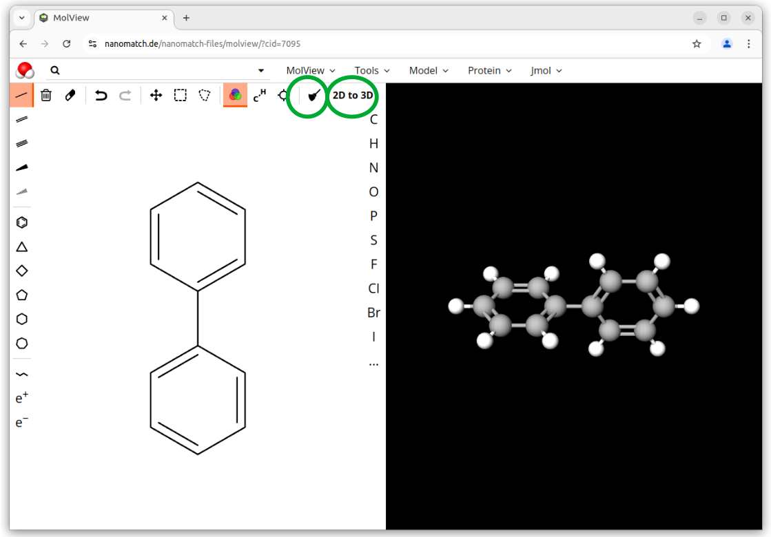
.mol (e.g. as downloaded by MolView, see step 2)
.pbd
.mol2
.cml
Note
To ensure that existing files are properly formatted, or in case MolPrep crashes due to incorrect input format, we recommend to convert the input using openbabel:
<your_input_format> can be any format accepted by openbabel, such as mol2, pdb, xyz, or simply a smiles-code or InChI, with <your_input_molecule> being the filename of the input file or simply the string for smiles or InChI. Check the Open Babel User Guide for reference.
Note
If you generated an initial 3D-structure from smiles or InChI, double check that the initial conformation is reasonable, e. g. by visualization with jmol.
If you don’t have any input for your molecule yet, a good starting point are drawing tools such as MolView. In the following we use MolView as an example.
Drag&Drop the modules MolPrep, Deposit and ESAnalysis from the top left panel into the middle workflow panel
into a linear workflow and arrange as depicted below. Double click on each module to adapt settings and allocate
resources for each simulation step.
Note
If you are unfamiliar with the setup of workflows, the Quick Start Guide may be a good starting point.
To simulate a pristine layer we construct a linear worklfow in SimStack comprising MolPrep, Deposit3 and ESAnalysis, as depicted in the above figure.
MolPrep:
Load an input file from your hard drive using the button right next to the input field Input Molecule File.
Deposit:
Adjust settings in the SimulationParameters Tab as described in Settings and Options, specifically box size or number of molecules, depending on your purpose.
Switch to the Molecules Tab. Use the rightmost buttons next to the Molecule and Forcefield input fields to load MolPrep/outputs/molecule.pdb and MolPrep/outputs/molecule_forcefield.spf, respectively.
ESAnalysis:
Use the rightmost button next to the Morphology input field to load Deposit3/outputs/structurePBC.cml.
Depending on the required output, adjust the Compute X options in the General Settings panel
Depending on the settings of 2., adapt Core Shell definition and Shell for Disorder and Couplings
Switch to the Engines Tab and set Memory per CPU (MB).
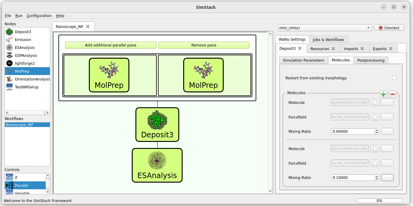
To simulate a guest-host systems, we need to combine two molecules in a single deposition:
Use a Parallel control from the Controls panel (bottom left) and click Add additional parallel pane.
Add one MolPrep module to each of the panes.
Add Deposit3 and ESAnalysis after the Parallel control.
Your workflow should look like this:
MolPrep:
Load the input (mol2) for the two molecules you would like to combine in the thin film into the two MolPrep modules.
Deposit:
Adjust settings in the SimulationParameters Tab as described in Settings and Options, specifically box size or number of molecules, depending on your purpose.
Switch to the Molecules Tab.
Press the + button to add the input for a second molecule.
First molecule: use the rightmost buttons next to the Molecule and Forcefield input fields to load Parallel/0/MolPrep/outputs/molecule.pdb and Parallel/0/MolPrep/outputs/molecule_forcefield.spf, respectively.
Second molecule: use the rightmost buttons next to the Molecule and Forcefield input fields to load Parallel/1/MolPrep/outputs/molecule.pdb and Parallel/1/MolPrep/outputs/molecule_forcefield.spf, respectively. Note the `1` in contrast to `0` in step b.
Adjust concentrations for your purpose.
ESAnalysis:
Use the rightmost button next to the Morphology input field to load Deposit3/outputs/structurePBC.cml.
Depending on the required output, adjust the Compute X options in the General Settings panel
Depending on the settings of 2., adapt the following:
Core Shell:
To compute absolute IP and EA in a mixed morphology for all species with sufficient accuracy, we recommend to set
Shell size defined by: Number of Molecules of each Type
Number of molecules: >= 2
Alternatively, if you are interested in the IP or EA of a few specific guest molecules in a host matrix, you can provide the list of molecule IDs. Note that for this purpose, you need to design the workflow up to Deposit, identify the respecitve IDs in the resulting structurePBC.cml and subsequently run ESAnalysis in a separate workflow with structurePBC.cml loaded from the hard drive.
Shell for Disorder and Couplings:
Accuracy of computed disorder depends heavily on the sample size. Keep in mind that for low concentrations, a large total number of molecules may be required in the disorder shell.
Switch to the Engines Tab and set Memory per CPU (MB).
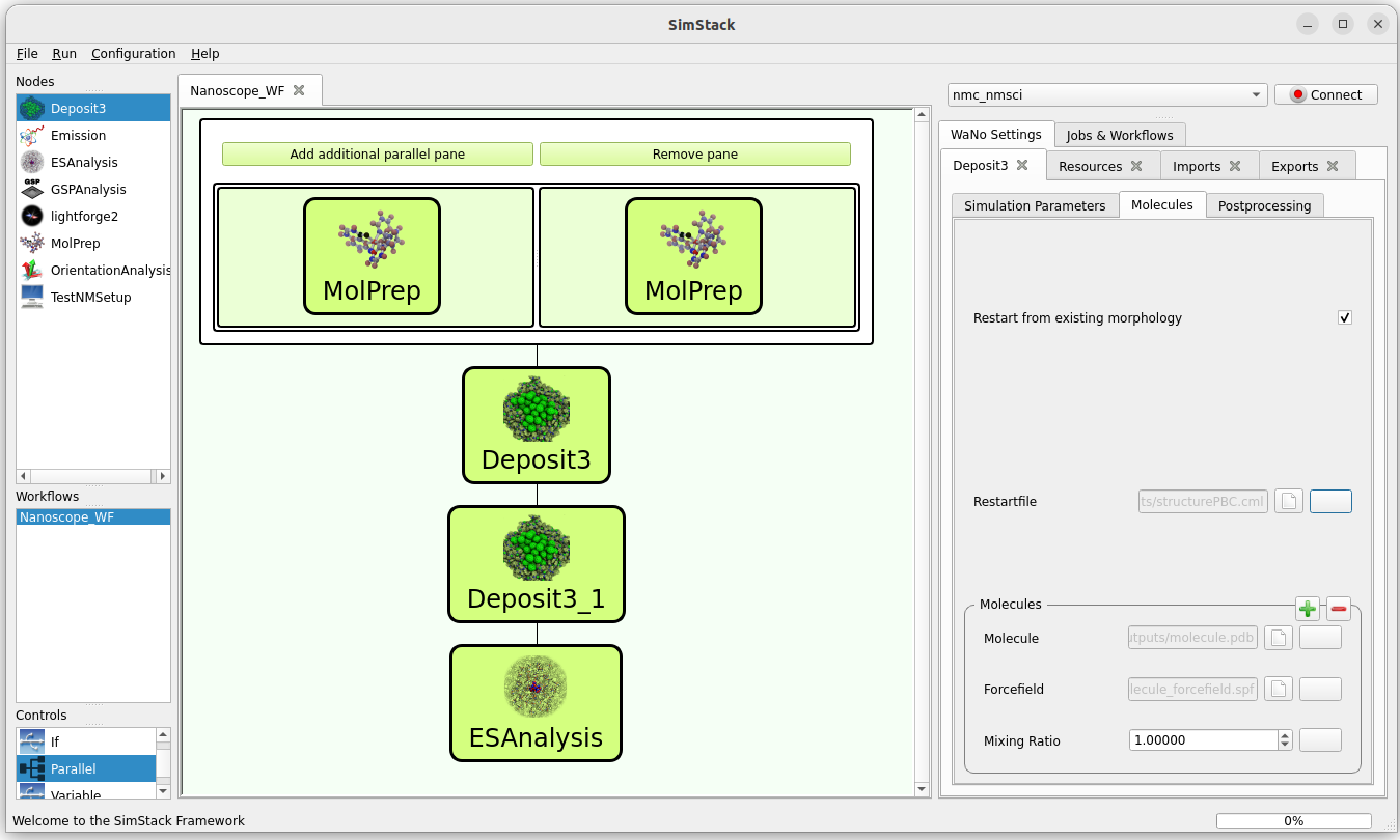
c. Simulation of a Multi-Layer Films and Interfaces
For an interface, we use the Parallel control to compute input for all molecules, but use multiple Deposit modules in sequence to deposit materials layer by layer:
Use a Parallel control from the Controls panel (bottom left) and click Add additional parallel pane. Add as many materials as you need in your multi-layer stack.
Add one MolPrep module to each of the panes.
Add multiple Deposit3 modules after the Parallel control in linear sequence.
Add ESAnalysis after the last Deposit3 module.
Your workflow should look like this:
MolPrep:
Load the input (mol2) for the two molecules you would like to combine in the thin film into the two MolPrep modules.
Deposit modules:
Adjust settings in the SimulationParametersTab as described in Settings and Options. Specifically, set the same total box height for all deposition steps.
Warning
All Deposit modules must have the same box dimensions. Make sure that, for all deposition steps:
X [A] and Y [A] are the same value
Set total box height for multilayer is enabled
Total Z [A] is the same value
Switch to the Molecules Tab. Use the rightmost buttons next to the Molecule and Forcefield input fields to load Parallel/X/MolPrep/outputs/molecule.pdb and Parallel/X/MolPrep/outputs/molecule_forcefield.spf, respectively. Adjust X depending on which material you would like to have in your layer.
For all Deposit modules except the first:
Enable Restart from existing morphology.
Use the button rightmost of the Restartfile input field to load the restartfile from the preceeding Deposit module, e. g. Deposit3/outputs/restartfile.zip. See the above figure for reference.
ESAnalysis:
Use the rightmost button next to the Morphology input field to load Deposit3_1/outputs/structurePBC.cml. If you have more than two layers, substitute Deposit3_1 with the last Deposit3 module in line.
Depending on the required output, adjust the Compute X options in the General Settings panel
Depending on the settings of 2., adapt the following:
Core Shell:
To compute absolute IP and EA in a mixed morphology for all species with sufficient accuracy, we recommend to set
Shell size defined by: Number of Molecules of each Type
Number of molecules: >= 2
Alternatively, if you are interested in the IP or EA of a few specific molecules, e.g. near an interface, you can provide the list of molecule IDs. Note that for this purpose, you need to design the workflow up to Deposit, identify the respecitve IDs in the resulting structurePBC.cml and subsequently run ESAnalysis in a separate workflow with structurePBC.cml loaded from the hard drive.
Shell for Disorder and Couplings:
The disorder shell is defined as N molecules closest to the center of the morphology. Depending on your layer setup, not all species may be well represented. We recommend to compute disorder in separate morphologies layer by layer.
Switch to the Engines Tab and set Memory per CPU (MB)
To compute the spontaneous orientation potential (SOP), also called giant surface potential (GSP) of a deposited thin film, add the GSPAnalysis module as depicted in the figure below. An example study is available in the publications: Built-In Potentials Induced by Molecular Order in Amorphous Organic Thin Films
In the GSPAnalysis WaNo adapt the following settings:
Morphology: load Deposit3/outputs/structure.cml (note: not structurePBC.cml from the preceding Deposit module
Forcefield: load MolPrep/outputs/molecule_forcefield.spf from the preceding MolPrep module
BoxSize: set the box size of your morphology in x- and y-direction, i.e. two times the settings Lx or Ly set in Deposit.
Note
GSPAnalysis only works for morphologies with Lx=Ly
Note
You can run the GSPAnalysis not only on pristine morphologies, but also on mixed systems. In this case, provide the merged.spf file from the Deposit module as input for Forcefield.
Note
In the above setup, vacuum ESP charges from MolPrep are used to compute GSP. You can also compute GSP based on charges equilibrated for the full morphology. A tutorial on how to do this will be supplied shortly.
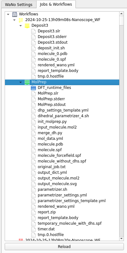
You can monitor the progress of your workflow with the Jobs&Workflows tab in the right panel of SimStack:
Navigate to the Jobs&Workflows tab on the right panel.
Expand Workflows (double click) and locate your submitted workflow (identified by timestamp if necessary).
Monitor the status of the workflow and the contained modules:
Green: Completed successfully
Yellow: Currently running
Red: Encountered an error
Double-click on a module to view logs, output files, and detailed status.
Note
Modules are only listed in this view once they have been started, i.e. when the predecessing module was finished successfully.
Once modules have completed successfully, you can download and view results by double-clicking on the modules and then the respective files in the Jobs&Workflows tab. Refer to Computed Properties for reference.